Covid Sequence Clustering
In this project, I compare machine learning techniques for clustering of SARS-CoV-2 cDNA sequences by variants.
At this point the whole world has had a crash course in virology, but to recap, the SARS-CoV-2 virus is an RNA virus. These types of viruses often mutate, due to the relative instability of RNA sequences. This results in many strains of the virus, some of which are more infectious than others.
For those who want to dive deeper into the nitty-gritty details, you can find the notebooks in the GitHub repository.
The Challenge
There are two items we need to address with clustering of cDNA sequences. First, we need to find a way to compare the sequences. Second, we need to find a way to group the sequences. This is a classic unsupervised learning problem.
To challenge myself, I will implement clustering solutions I currently use. Typically I would first do a literature search to find state-of-the-art approaches, but want to solve this problem with my own approaches.
Also, I will avoid libraries like Biopython that are specifically designed for bioinformatics. Instead I will use raw python and numpy to manipulate sequences. For the linear algebra of the clustering techniques, I will use solely numpy and only use sklearn for some convenience functions. Again, this is to challenge myself to implement algorithms from scratch where I would typically use 3rd party libraries. This is reinventing the wheel, but sometimes it’s worth it to get that sense of accomplishment.
The Data
The data I have is multi-sequence alignment (MSA) of 400 SARS-CoV-2 sequences in a fasta file. The sequences are of complementary DNA, sequenced from viral RNA that has undergone reverse transcriptase. The sequences are from sample that originate from an unknown number of strains.
Each location of the sequences can have the four nucleotides A, C, G, or T. A position could also have a N if the nucleotide was indeterminate or a - if there was no sequence data at that position. The sequences have been aligned and fully conserved regions replaced with the symbol ..
The Method
To cluster the sequences, I first needed to clean the data. Next I needed to find a similarity measure to compare the sequences. Then I used a variety of clustering algorithms to group the sequences.
Data Cleaning
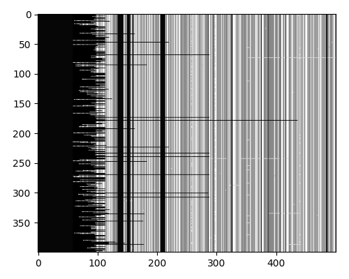
I used python to parse the fasta file. I then converted the 400 sequences into a numpy array with the characters converted to integers. This gave me a 400 x 34,044 array.
This left me with sequences that contained missing (-) or indeterminate (N) data. If a given MSA position had less that 5% missing data, I imputed the missing data with the most common nucleotide at that position. If a position had more than 5% missing data, I removed the sequence from the dataset. This resulted with the typical sequence having 1-2% of the positions imputed.
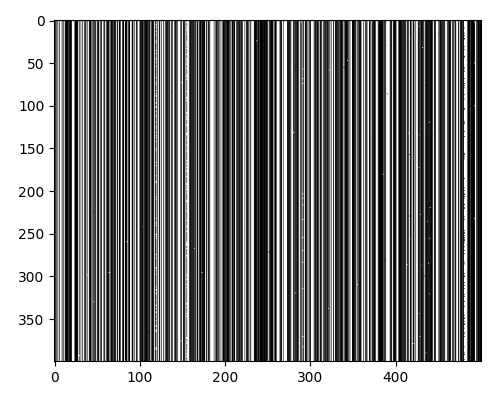
At this point I also dropped all fully conserved positions (.), as they would not contribute to the clustering. This left me with a 400 x 17,463 array.
Next I calculated the entropy of the MSA for each position. This gives us an idea of how variable the sequence positions are. We get a sense of baseline noise of random mutations, as well as positions that have low conservation across major strains.
Note for the entropy calculation, I used \(log_4\) to account for the number of nucleotides, although hte convention is \(log_2\) for bits. To me this makes more sense, since DNA is quaternary, not binary.
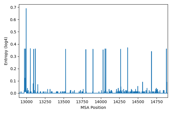
Most positions are fully conserved with an entropy of 0. Some positions have small entropy values, representing positions that are conserved with occasional random mutations. Some positions have high entropy values, representing positions that are highly variable and may indicate mutations across major strains.
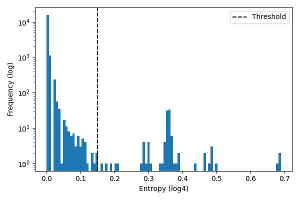
Next I plotted a histogram of the entropy values to visualize the random mutations versus the major strain mutations. We can see below the distribution is multimodal. I put a cutoff threshold at 0.145, which is at the right tail of the random mutation distribution. This cutoff will be used to filter out positions that are not conserved across major strains. Future work could look at fitting a mixture model to the entropy distribution to find the optimal cutoff.
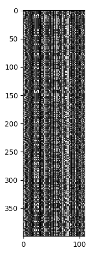
After trimming the MSA to remove low entropy positions, I was left with a 400 x 110 array. This is a good size for clustering, as it is a good balance between having enough data to find clusters and not having too much data to be computationally expensive.
Similarity Measure
Now onto the exciting world of similarity measures! The next step in clustering will be to generate a similarity data structure from the sequence data. I will use the Hamming distance as the distance metric. This is a good distance metric for sequences since it works with discrete categorical data. For a pair of sequences, the Hamming distance will be the number of positions where the sequences have different nucleotides.
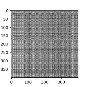
The trick with Hamming distance is that it gives us a relative similarity between sequence pairs, but not on an absolute scale. We can address this issue by building a graph of the sequences, using the similarity as edge weights. This gives us a good sense of the local structure of the data. We will represent the graph as an adjacency matrix.
To provide cleaner results, I made the dense adjacency matrix sparse. Only the nearest 75 neighbors to a sequence node are retained. The rest are dropped.
Clustering Algorithms
The next step is to cluster the graph. I have two ideas for this, using different perspectives.
The first perspective is to use linear algebra to find a low dimensional representation. We can cluster on the eigenvectors with the lowest eigenvalues. This approach is called spectral clustering.
The second perspective is to treat the neighborhood graph as a low dimensional manifold in high-dimensional space. I will use the manifold learning algorithm ISOMAP to calculate a low-dimensional representation that preserves the geodesic distances and then cluster.
For the clustering algorithm, I will use \(k\)-means. I will also implement my own version of \(k\)-means from scratch in numpy to challenge myself.
Spectral Clustering
For spectral clustering I will first convert the adjacency matrix into a Laplacian matrix, which allows use to have at least one eigenvalue equal to zero.
I tried both the standard Laplacian, \(L = D - A\), and the normalized Laplacian, \(L = D^{-\frac{1}{2}} \cdot A \cdot D^{-\frac{1}{2}}\). Here \(D\) is the distance matrix which is a diagonal matrix that sums the weights of the adjacency matrix. I found the standard Laplacian worked better for this application.
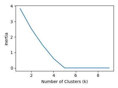
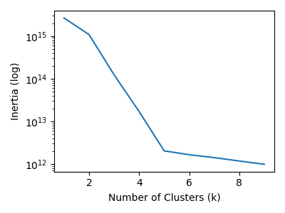
For clustering, I used classic \(k\)-means. I validated the choice of \(k\) with visualizations of the elbow diagram, adjacency matrix, MSA sequences, and eigenvectors.
Clustering with ISOMAP
For the ISOMAP, I calculated the geodesic distance matrix \(D2\) from the graph by finding the shortest path between each pair of sequences. I next center the matrix using the centering matrix \(H\). We then select the \(n\) largest eigenvalues to perform multidimensional reductions (MDS), resulting in a reduced representation matrix \(Z\).
I cluster the matrix \(Z\) with \(k\)-means and then validate the clusters like with spectral clustering.
The Results
Both approaches find 5 major strains of SARS-CoV-2 sequences. As we increase the \(k\) value, the major strains clusters get subdivided into outlier sequences and sub-strain clusters.
Spectral Clustering
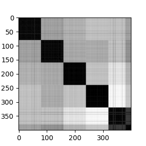
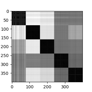
If we look at the adjacency matrix for spectral clustering, we can see the effects of the number of clusters. It make five clusters well. Going beyond five clusters, we see the most heterogenous cluster breaking into into sub-clusters.

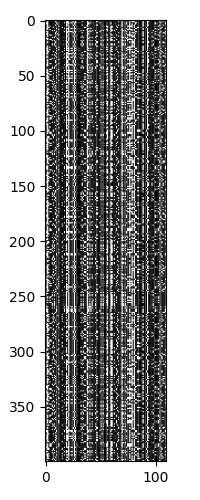
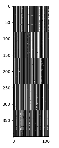
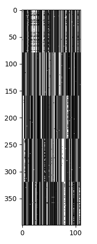
Looking at the sequences, we again see that there are 5 major strains, with each strain having different levels of heterogeneity.


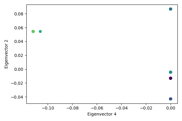
We can also look at the clusters in the reduced spectral space. Eigenvectors 1 and 2 show good separation among the 5 clusters. On eigenvector 4, we see separation of one cluster into sub-clusters.

ISOMAP
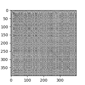
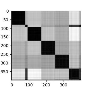
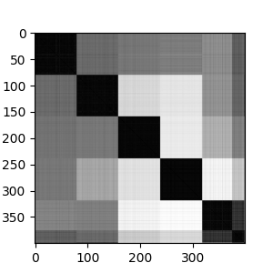
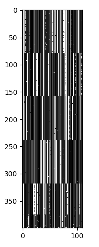
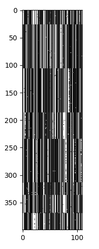
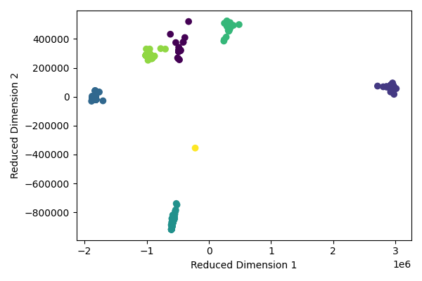
The ISOMAP results are similar to the spectral clustering result. We see 5 major strains, with each strain having different levels of heterogeneity. At \(k\)=9, the ISOMAP does a better job of separating the sub-strains, as we can see in the geodesic distance matrix below.

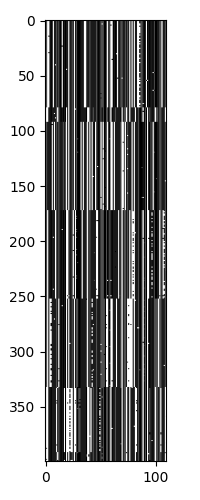
Next we can see the clustering of the sequences.
We can visualize the clusters in the reduced ISOMAP space. We see good separation among the 5 clusters, with further separation of some sub-clusters when \(k\)=7.
Conclusion
Both the spectral clustering and ISOMAP approaches worked well for clustering the SARS-CoV-2 sequences. Both approaches found 5 major strains, with each strain having different levels of heterogeneity. The ISOMAP approach did a better job of separating the sub-strains. Further validation could be performed by using labeled data with strain information.
Further work could be done to identify the sensitive of the results to the data cleaning thresholds. Also, the entropy cutoff could be optimized by fitting a mixture model to the entropy distribution. Finally, the clustering algorithms could be optimized for speed and memory usage.
The clustering of the strains also raises questions of phylogeny. The clustering could be used to build a phylogenetic tree of the strains. This could be done by using the Hamming distance as a measure of genetic distance between the strains. The tree could be built using a variety of phylogenetic tree algorithms, such as UPGMA or neighbor joining. Or we could drop clustering altogether and model the viral evolution as part of a Ornstein-Uhlenbeck process with stochastic differential equations.
I hope this project has given you a good overview of how to cluster cDNA sequences. If you have any questions or suggestions, please feel free to reach out to me.